Case Study: Detecting Defects Without Deep Learning

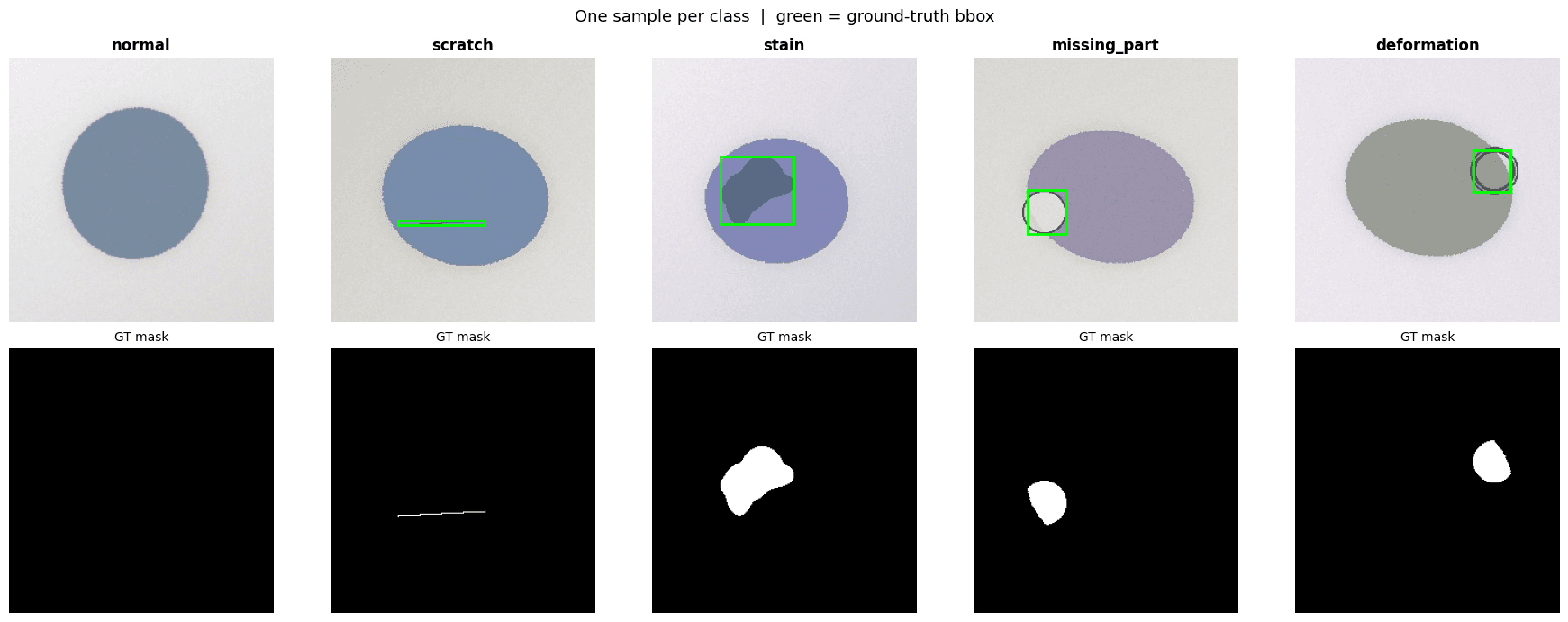
The problem: a mini industrial quality-control task with five defect classes — normal, scratch, stain, missing_part, deformation — on 256x256 product images, and only 75 labeled examples to learn from. The obvious modern instinct is to reach for a CNN. I didn't, and the results back that decision up.

Why not deep learning With 15 images per class, any convolutional network would essentially memorize the training set rather than learn generalizable features. The dataset is also synthetic, with defects that have clear, consistent visual signatures — exactly the kind of structure that classical computer vision features are good at capturing, without needing thousands of examples to discover it from scratch.

The pipeline

1. Segmentation: Top-Hat and Black-Hat morphological filtering combined with Canny edge detection isolates the candidate defect region in each image.
2. Feature extraction: from that region, 10 numerical features are computed — area, aspect ratio, fill ratio, brightness, relative brightness, distance from center, saturation, solidity, perimeter ratio, and bounding-box area.
3. Classification: a 200-tree Random Forest is trained on those 10 features.
4. Localization: the same segmentation bounding box is reused for defect localization, corrected with a per-class shrink factor learned from the training set, since raw segmentation tends to overestimate defect size at blurry transition pixels.

One detector, not five An earlier version of this project used class-specific detectors: a Hough line transform for scratches, LAB color-deviation analysis for stains, and convex-hull differencing for edge defects like missing parts and deformation. I benchmarked these against a single generic detector (the Top-Hat/Black-Hat + Canny approach above) on the validation set. The generic method won for every class — including a jump from 0.0 to 0.816 IoU on deformation, where the convex-hull approach failed outright. That was a useful reminder that a well-tuned general method can beat several specialized ones, and it is far easier to maintain one pipeline than five.

Results Macro F1 reached 0.96 on validation and 0.97 on the hidden test set. Mean IoU for localization was 0.72 on validation and 0.74 on test. The combined final score (weighted 65% macro-F1, 25% mean-IoU, 10% accuracy) was 0.90 on validation and 0.91 on the hidden test set. All of this trained in seconds, on a CPU.

The per-sample IoU breakdown tells a more honest story than the averages alone: some individual scratch predictions scored close to 0 IoU (thin, low-contrast defects are genuinely hard to localize precisely), while missing_part and stain predictions were consistently strong. That spread is useful information that a single averaged metric hides — worth surfacing in any evaluation, not just this one.

Takeaway Not every computer vision problem needs a neural network. When the dataset is small and the defect signatures are visually consistent, a handful of well-chosen features and a Random Forest can outperform a CNN, train in seconds, and be far easier to debug and explain.