Breast Cancer Diagnosis Prediction: A Comparative Analysis of KNN and SVM Algorithms
A machine learning project predicting whether a breast tumor is benign or malignant using K-Nearest Neighbors and Support Vector Machines, with full hyperparameter tuning and performance comparison. Developed as the final project for the Huawei Student Developers x Turkiye Yapay Zeka Akademisi Data Science and Machine Learning Bootcamp.
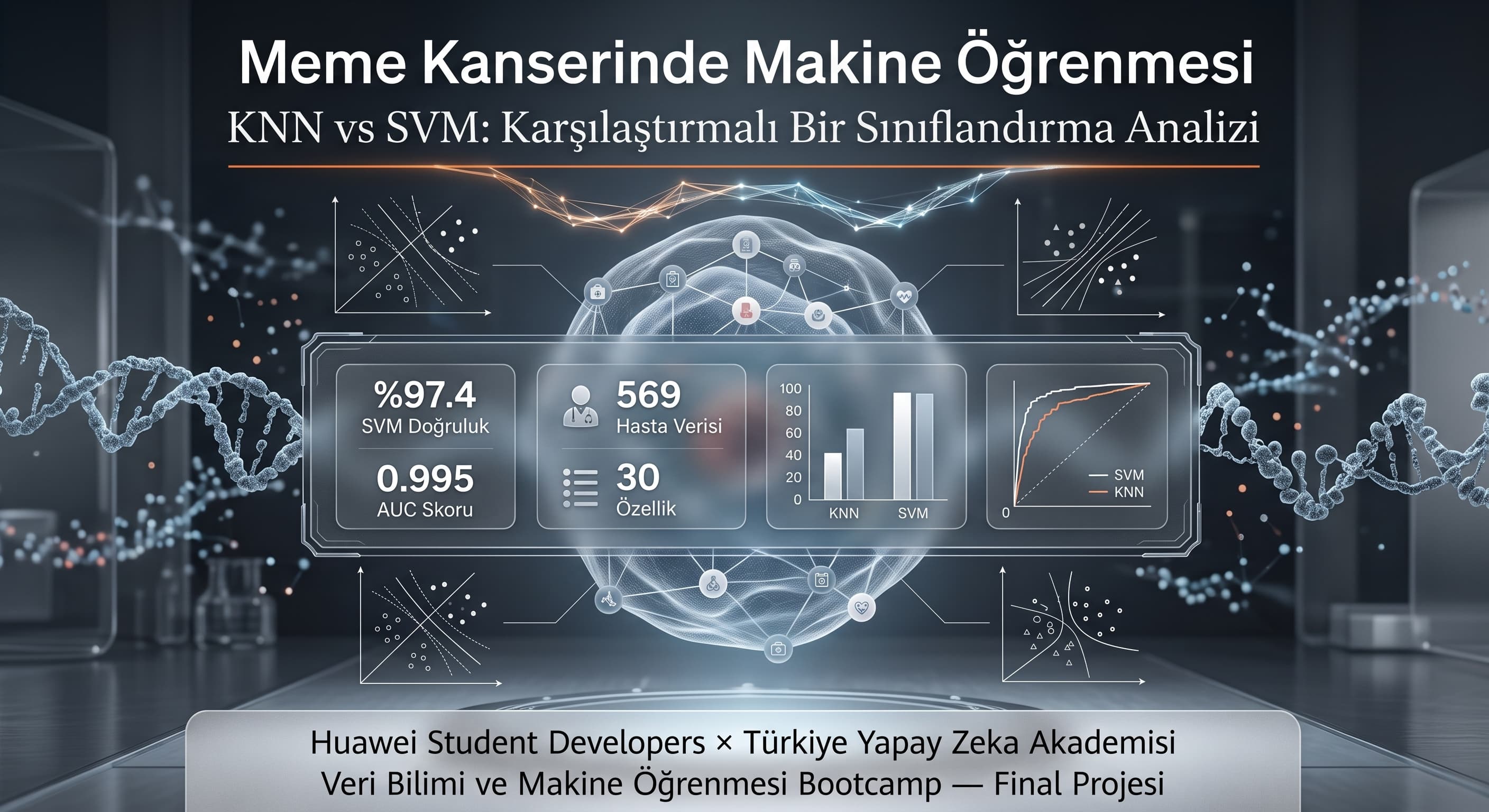
Breast Cancer Diagnosis Prediction: KNN vs SVM
Breast cancer is one of the most common cancers among women worldwide, and early diagnosis directly affects treatment success. In this article, I'm sharing a machine learning project I developed as the final project for the Huawei Student Developers x Turkiye Yapay Zeka Akademisi Data Science and Machine Learning Bootcamp.
The project addresses a simple but real-world question: can we predict whether a breast tumor is benign or malignant based on measurements taken from cell nuclei?
To answer this, I trained two different classification algorithms — K-Nearest Neighbors (KNN) and Support Vector Machines (SVM) — tuned their hyperparameters, and compared their performance across several metrics.
Objective and Problem Definition
This is a binary classification problem. We have 30 numerical measurements derived from biopsied cell nuclei, and each observation is labeled as either benign or malignant.
My goal wasn't just to achieve high accuracy. I also wanted to observe how two fundamentally different algorithm families (distance-based KNN vs. margin-based SVM) behave on the same problem, demonstrate the concrete impact of hyperparameter tuning, and highlight why accuracy alone is insufficient in a sensitive domain like healthcare — where precision and recall matter just as much.
Dataset
This project uses the Breast Cancer Wisconsin (Diagnostic) Dataset — 569 observations, 30 numerical features. Each feature describes a characteristic of the cell nucleus (radius, texture, perimeter, area, smoothness, compactness, concavity, concave points, symmetry, fractal dimension), expressed as three statistics: mean, standard error, and worst value.
I chose this dataset because it's well-established and widely used on Kaggle, fully numerical, and addresses a meaningful real-world problem.
Data Preparation and Exploratory Analysis
The first step is always understanding the data. After inspecting the CSV downloaded from Kaggle, I found two non-informative columns: id (patient identifier) and Unnamed: 32 (a completely empty column), both of which I removed. None of the remaining 30 feature columns had missing values — this significantly simplified the data cleaning process.
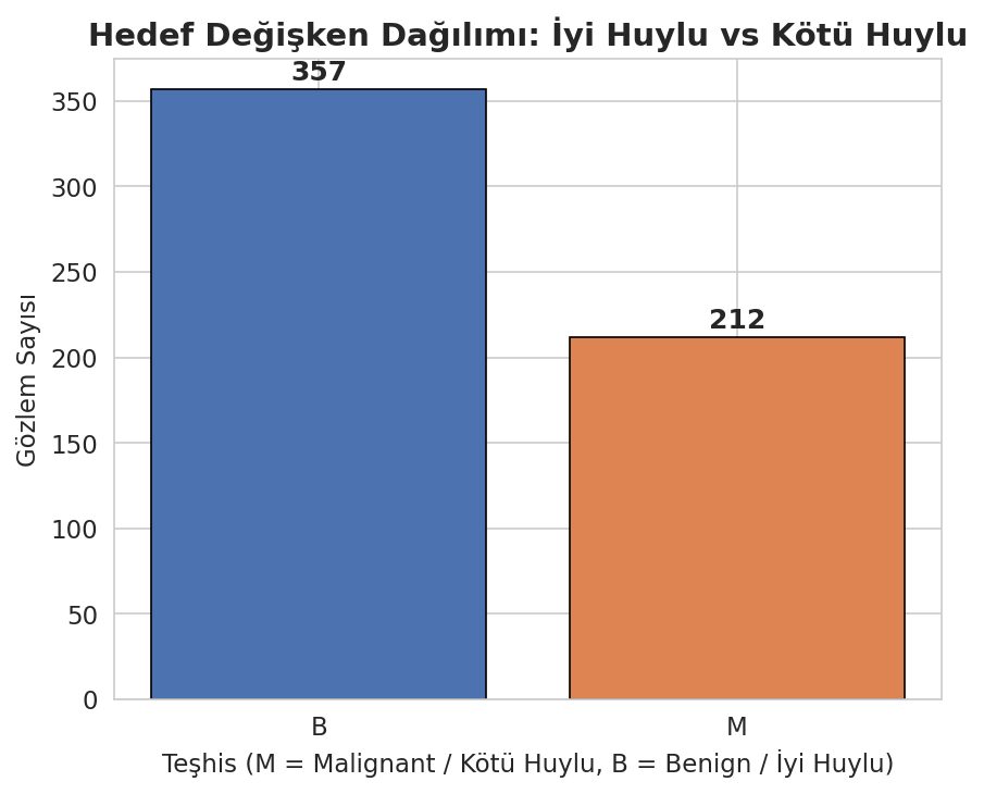
Target distribution: Class imbalance can cause a model to show misleadingly high accuracy if ignored. Here: 357 benign cases (62.7%), 212 malignant cases (37.3%). There was no severe imbalance, so no additional balancing technique was needed.
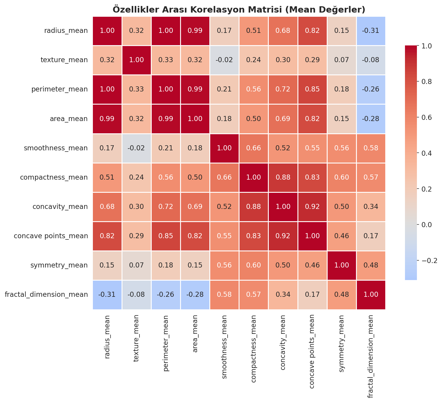
Correlation analysis: I built a correlation matrix to examine relationships between features. Size-related features like radius_mean, perimeter_mean, and area_mean showed near-perfect correlation (up to 0.99) — which makes mathematical sense, since a larger radius naturally leads to a larger perimeter and area. In contrast, texture_mean showed a much weaker relationship with other features, indicating it carries information independent of cell size.
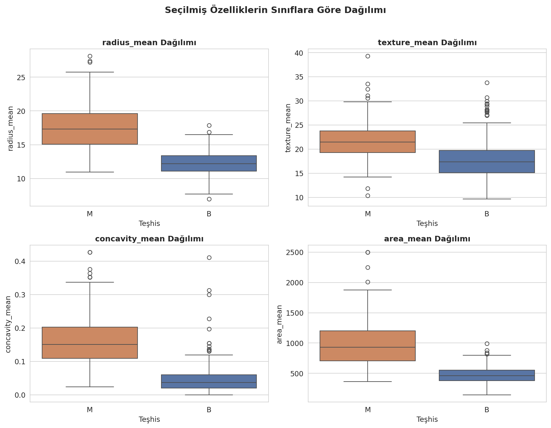
Feature distributions by class: Using boxplots, I examined which features showed the clearest separation between the two classes. For features like radius_mean and area_mean, the boxes for malignant and benign cases barely overlapped — for area_mean specifically, the median for malignant cases was roughly double that of benign cases. texture_mean, on the other hand, showed much more overlap between the two groups.
Scaling: Since both KNN and SVM are distance/margin-based algorithms, I standardized all features to have mean 0 and standard deviation 1 using StandardScaler. I also split the data into 80% training (455 samples) / 20% testing (114 samples), preserving class proportions via stratification.
Model 1: K-Nearest Neighbors (KNN)
KNN's logic is quite intuitive: for a new observation, it looks at its K nearest neighbors and predicts the class based on their majority vote. The most critical hyperparameter is K — to find the best value, I tested every K from 1 to 30 using 5-fold cross-validation. (A great video explaining how KNN works)
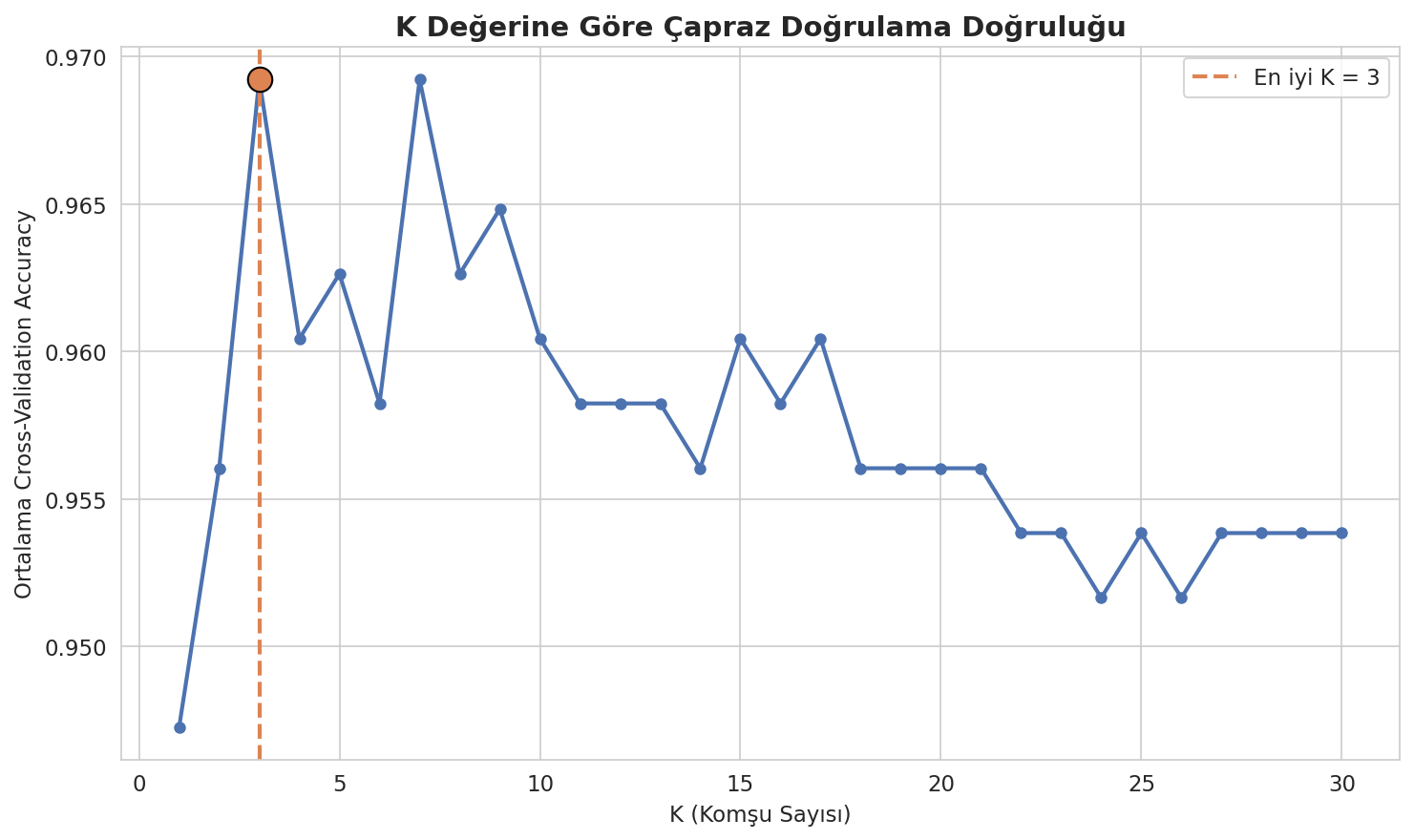
This analysis found the best K value to be 3 (cross-validation accuracy: 96.9%). At K=1 the model was overly "sensitive" and showed lower performance, while as K increased the model became more "generalized" and performance gradually declined.
Model 2: Support Vector Machines (SVM)
SVM works on a different principle: it tries to find the boundary that separates the two classes with the widest possible margin. For data that isn't linearly separable, it can use the kernel trick to project data into a higher-dimensional space where it becomes separable. (A video explaining how SVM works and the kernel trick)
I used GridSearchCV to optimize these hyperparameters (C, kernel, gamma). The result: the best parameters were C=1, kernel=rbf, gamma=scale (cross-validation accuracy: 97.6%). The fact that the rbf kernel performed best suggests the boundary between classes isn't entirely linear.
Results and Comparison
I evaluated both models on the test set using accuracy, precision, recall, and F1-score:
| Model | Accuracy | Precision | Recall | F1-Score | AUC |
|---|---|---|---|---|---|
| KNN (K=3) | 93.9% | 97.3% | 85.7% | 0.911 | 0.982 |
| SVM (rbf, C=1) | 97.4% | 100.0% | 92.9% | 0.963 | 0.995 |
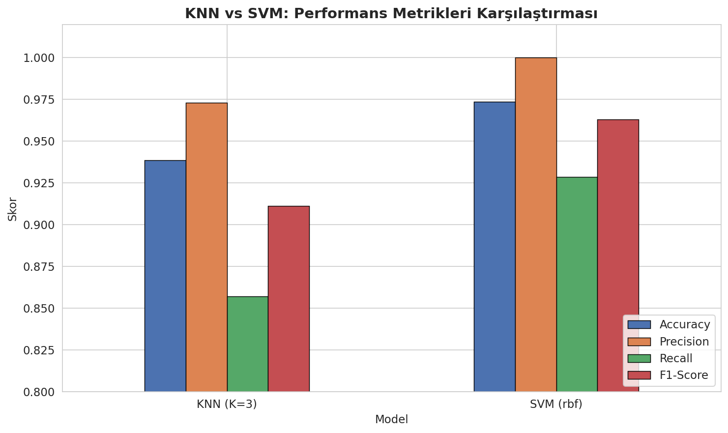
SVM outperformed KNN across every metric. The most notable difference was in recall: KNN correctly caught only 85.7% of malignant cases, while SVM caught 92.9%.
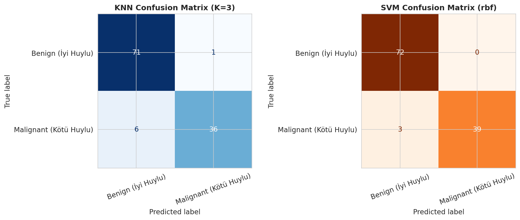
The confusion matrix comparison makes this difference much more concrete: out of 42 malignant cases in the test set, KNN missed 6, while SVM missed only 3. SVM also correctly classified all 72 benign cases, with zero false alarms.
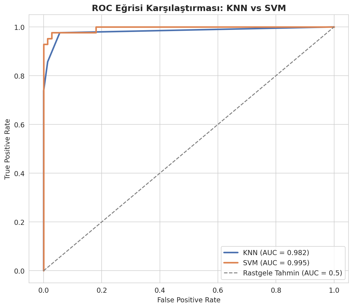
ROC curve and AUC: Both models achieved AUC scores very close to perfect (KNN: 0.982, SVM: 0.995). Put simply: given a random malignant and a random benign case, SVM can correctly rank them 99.5% of the time — an almost flawless discriminative ability.
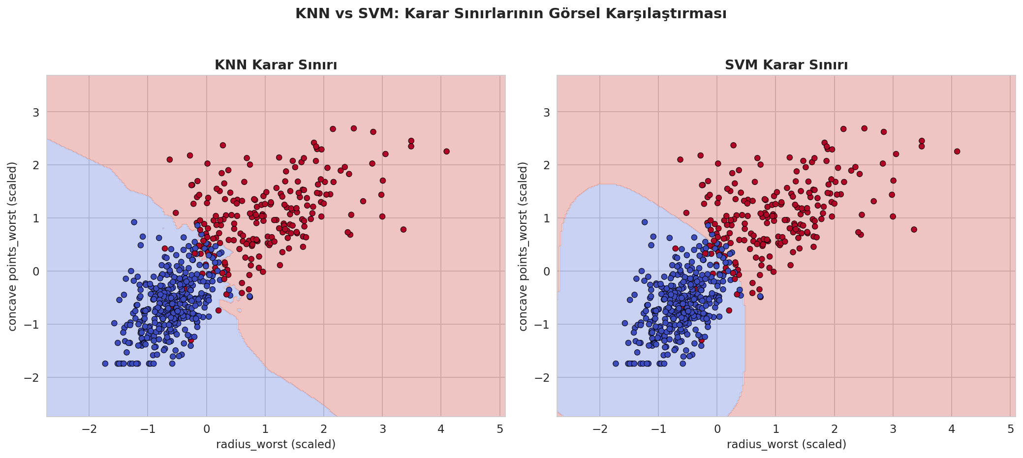
Decision boundary visualization: To make the models' "thinking" more tangible, I created a 2D decision boundary visualization using the two most discriminative features. This clearly shows the philosophical difference between the two algorithms: KNN draws a more "irregular/local" boundary based on the local density of the data, while SVM draws a smoother, more general boundary.
Key Takeaways
The most important lessons from this project:
-
Feature scaling is absolutely essential for distance/margin-based algorithms. In my earlier quick tests without StandardScaler, model performance dropped noticeably with unscaled data.
-
Hyperparameter tuning genuinely makes a difference. Testing all K values from 1 to 30, I found K=3 gave a much better cross-validation performance than a default K value. Similarly, using GridSearchCV to find the right kernel and C value for SVM improved its generalization.
-
There is no universally "best" algorithm — it depends on the dataset. SVM led on every metric here because the class boundary had a mildly non-linear structure. This doesn't mean SVM is always better than KNN — the result could reverse on a different dataset.
-
Accuracy alone isn't enough, especially in sensitive domains like healthcare. Precision, recall, and confusion matrices are essential for understanding what kind of errors a model actually makes. Although the accuracy gap between the two models (93.9% vs 97.4%) looks small, the confusion matrix revealed it corresponds to a concrete, meaningful difference: 3 fewer missed malignant cases.
Future Directions
This project was built under a tight bootcamp deadline, but there are several directions for future work: adding ensemble methods like Random Forest or Gradient Boosting to the comparison, applying feature selection techniques to improve interpretability, testing generalizability on data from different hospitals or populations, and using explainability techniques like SHAP or LIME to interpret individual predictions in more depth.
Closing Thoughts
This project was developed as the final project for the Huawei Student Developers x Turkiye Yapay Zeka Akademisi Data Science and Machine Learning Bootcamp. Throughout the process, I got to experience both the practical application of classic machine learning algorithms and how a data science project runs end-to-end. Working with healthcare data was also a reminder of how carefully and responsibly machine learning models need to be developed for real-world use.
The full code, visualizations, and detailed analysis are available via the GitHub, Kaggle, and Medium links above.
This project was developed as the final project for the Huawei Student Developers x Turkiye Yapay Zeka Akademisi Data Science and Machine Learning Bootcamp.